Hybrid LP-NLP Hydropower optimization model in pyomo

This is an object-oriented, hybrid linear-nonlinear programming hydropower optimization model for California. It is modeled in pyomo, high level optimization programming language. The model is capable of creating linear and nonlinear hydropower models. Since linear model is much faster than nonlinear, its results can be used as a initial solution (warmstart) for the nonlinear model. Linear model results can also be used as stand alone. When warmstart=True and both LP and NLP models run sequentially, initial primal variables from LP model are fed into NLP model, decreasing iterations for convergence and runtime.

Nonlinear model

The model represents nonlinearities of hydropower due to storage (so water head). Head is dynamically calculated as a polynomial function of storage. Polynomial functions are predetermined and plant-specific. Large-scale nonlinear solver ipopt is used to solve the problem.

ipopt documentation and solver options can be found at:

https://www.coin-or.org/Ipopt/documentation/documentation.html

Linear model

Unlike nonlinear model, head is not dynamically calculated. Unit benefits are predetermined based on maximum benefit from maximum storage and release. Large-scale nonlinear solvers glpk or cbc can be used to solve the problem. For linear model, unit price (slope) values c must be defined for storage and release. So, during LP preprocessing (network export process), for each time step, using scipy, a linear benefit surface (below) is fit to a nonlinear benefit curve (below), minimizing error due to fit. And then, unit price or slope values are obtained for the LP model.

from scipy import optimize # used to fit linear curve
def fun(x): # maximize r2
    benefit_linear = stx*x[0]+fly*x[1]
    SSE = np.sum((benefit_nonlinear-benefit_linear)**2)
    SST = np.sum((benefit_nonlinear-np.mean(benefit_nonlinear))**2)
    r2 = 1-SSE/SST
    return -r2
x0 = np.array([1,1])
res = optimize.fmin(fun,x0,disp=False)

Residuals

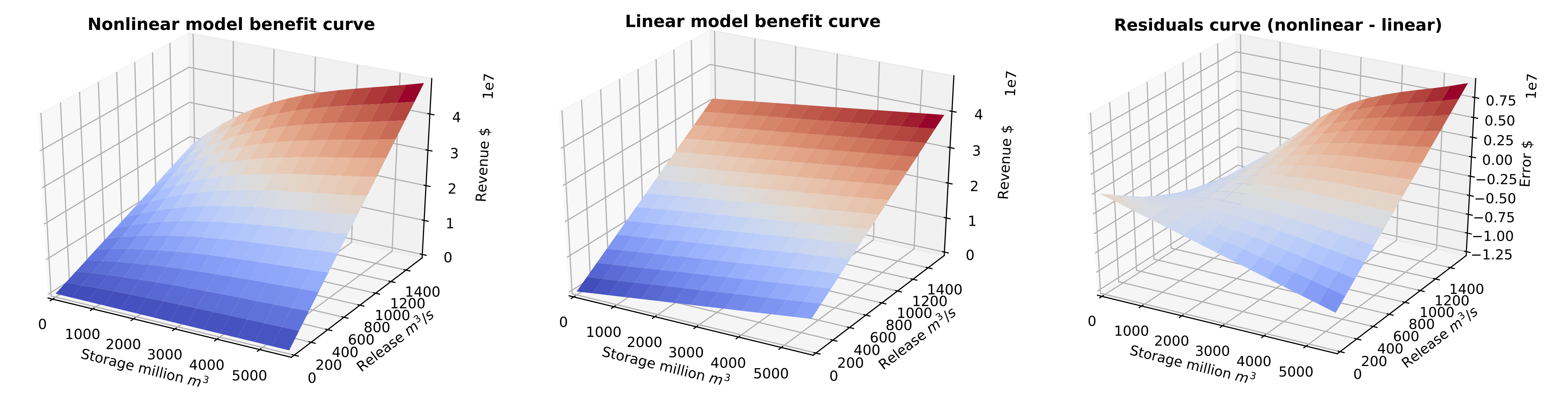
Error or residuals between nonlinear and linear benefits curve vary depending on storage and release. However, there is a region where residuals are zero; between (mid storage, max release) and (max storage, mid release).

Benefit curves for nonlinear and linear models and residuals

benefit_curves

Typical outputs:

flow_cms.csv releases and flows (cubic meter per second) on links
storage_million_m3.csv reservoir storages (million cubic meter)
dual_lower_flow.csv dual values on lower bound constraints for flow links
dual_lower_storage.csv dual values on lower bound constraints for storage links
dual_upper_flow.csv dual values on upper bound constraints for flow links
dual_upper_storage.csv dual values on upper bound constraints for storage links
dual_node.csv dual values on mass balance constraints
power.csv power (megawatt)
generation_MWh.csv power generation (megawatt hour)
revenue_$.csv power revenue (dollar)

Visualization

animation

WARM-STARTED solve

warmstart = True

Warmstart option improves runtime and feasiblity for Nonlinear Programming model by obtaining optimized decision variables from a previous feasible solution. If warm start option is enabled, the model is solved twice: first with initial (warmstart) values of variables and then updated suffix parameters from initial solve. Initial variable values (flow and storage) are obtained from unorganized_f.csv and unorganized_s.csv. So, the model must have solved in defined time-step (frequency) first. Otherwise, initial values will be zero even if warmstart = True. The idea is that first Linear Programming model is solved, then output decision variables are fed into Nonlinear Programming model to boost runtime and feasibility. The code can be modified to read initial decision variable values from a previous NLP model outputs (warmstart_path). Warmstart is not modeled with LP model since it is already fast enough.

Time-step selection

The model is flexible on time-step selection and supports several time-step options, ranging from hourly to annual. As long as input data has high resolution (or at least higher than desired time-step), during preprocessing data files are generated based od selected time-step. Currently price and flow data have hourly time-step, so the model can create hourly, daily, weekly, monthly or annual averages. Also, if overall_average=True, time-series are grouped based on selection. For example, overall_average=True and step=['H'], then the model will create average of all hours from 0 to 23. Finally, multiple time indices are supported. If overall_average=True and step=['A','H'], the model will create time-step for each year and hour between start and end time.

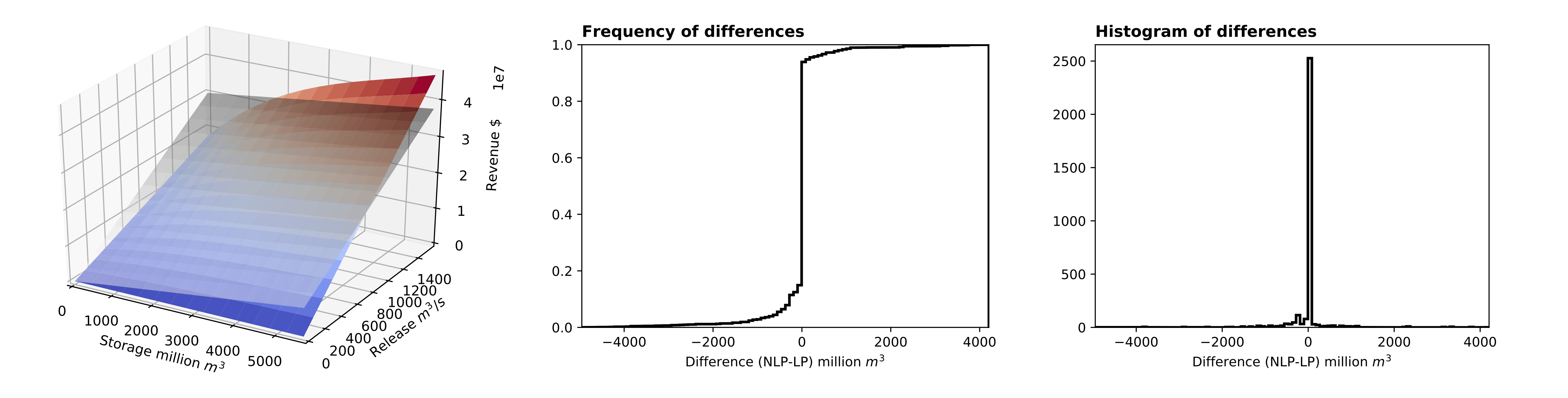
Errors between NLP and LP

Benefit curves drive operations for both NLP and LP models. While benefit curve and its function optimized and water head is dynamically calculated for NLP model, prescribed linear benefit curves are used for LP model. Differences between benefit curves (residuals) are discussed above. Due to residuals, errors on output decision variables occur.

errors

Network schematic

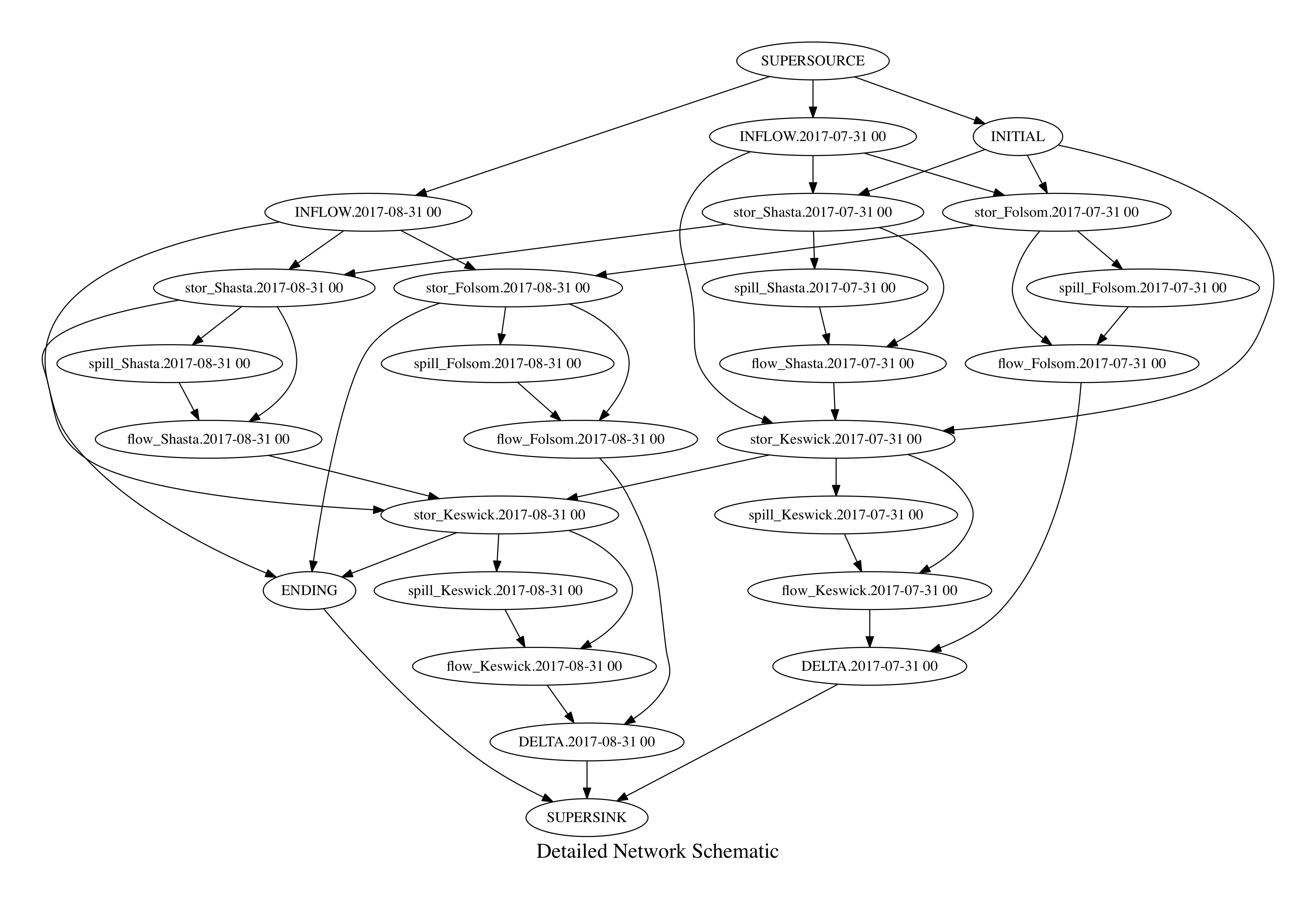
simplified network schematic

Detailed network schematic (multi-stage)

Detailed network

Dependencies

Required:

python programming language (Anaconda recommended)
pyomo library and pyomo extras
ipopt nonlinear programming solver
glpk or CBC linear programming solver

After installing Anaconda, pyomo and solvers can be installed by running the command:

conda install -c conda-forge pyomo pyomo.extras glpk ipopt

Optional:

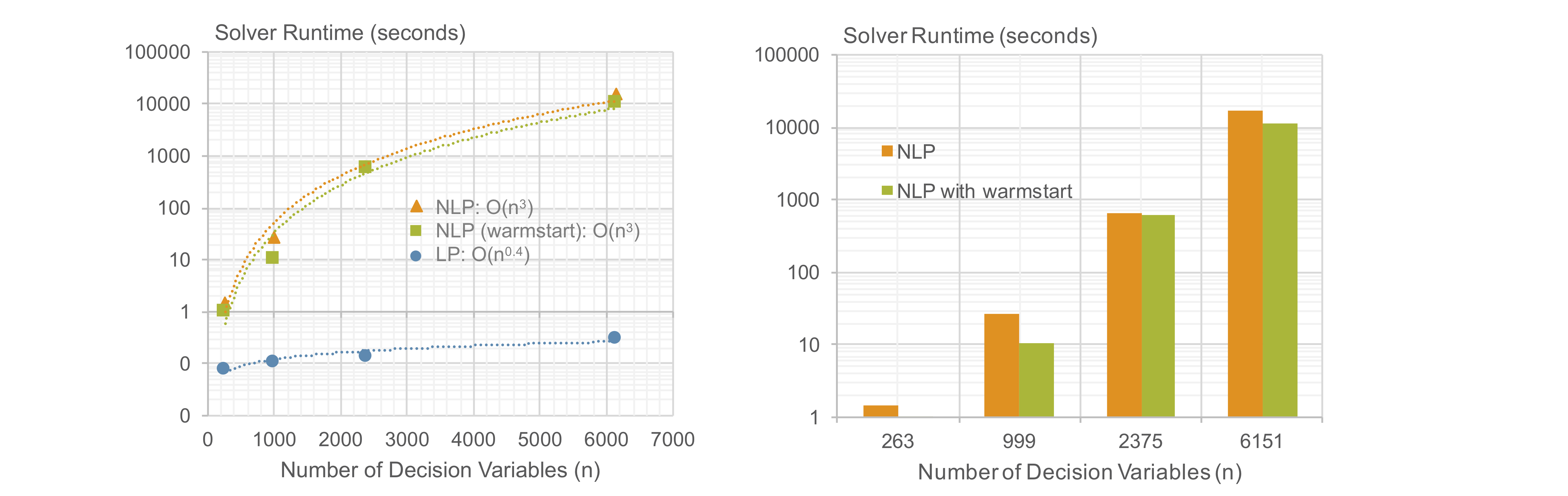
Basemap for displaying plants on a map
graphviz printing network schematic

Solver Runtime

Linear programming (LP) model runs significantly faster than nonlinear programming (NLP) model. Runtime (wall clock time) scalability for different number of decision variables are shown below on a semi-log scale. Runtime increases exponentially as number of decision variables increase. Although NLP and NLP warmstart models have similar orders of magnitude, O(n^3), overall warmstart option reduces runtime in all model sizes.

runtime

cProfile results for code performance

python -m cProfile main.py

This repository is greatly benefited from calvin

https://github.com/ucd-cws/calvin

hydropower_optimization

Hydropower optimization model in Pyomo